Isomorfismos: poda con automorfismos (3)
Cómo el orden refinamiento y la celda objetivo afectan al tamaño del árbol de particiones
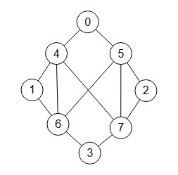
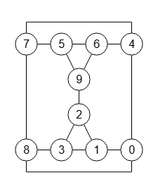
El objetivo principal del algoritmo de McKay con la implementación que llevo a cabo con getPartitionTree() es obtener el etiquetado canónico del grafo que se devuelve en el campo canonicalLabel del resultado. Pero también esta implementación me sirve para analizar y trazar la ejecución del árbol de particiones, automorfismos y cómo las opciones de ejecución pueden modificar el resultado. Para ver esto último tomaremos el grafo de la Figura, que puede importar en la aplicación con el archivo graph-sample-10.txt
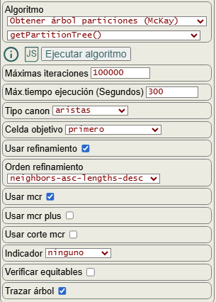
En la Figura vemos las opciones para ejecutar el algoritmo getPartitionTree(), de las que ya hablamos en un tema anterior.
Las opciones orden refinamiento ("orderRefine") y celda objetivo ("targetCell") son las que veremos en este tema, empezando por esta última.
Obtenemos el siguiente resultado:
Time: 2 ms

Obtener árbol particiones (McKay): {
"useRefine":true,
    "orderRefine":"neighbors-asc-lengths-desc",
    "targetCell":"first",
    "typeCanon":"edges",
    "useMcr":true,
    "useMcrPlus":false,
    "useMcrBreak":false,
    "typeIndicator":"none",
"timeTotal":2,"timeIni":0,"timeRef":0,
"iter":14,"refine":9,"indexTree":8,
"leaves":5,
"prunningMcr":2,"prunningMcrBreak":0,
"prunningIndicators":0,"prunningIndicators2":0,
"firstCanonicalPartition":[[0],[1],[2],[3],[7],[6],[5],[4]],
"firstCanon":false,
"canonicalPartition":[[1],[0],[3],[2],[7],[5],[6],[4]],
"firstCanonicalLabel":[[0,6],[0,7],[1,5],[1,7],[2,4],[2,6],[3,4],[3,5],[4,6],[4,7],[5,6],[5,7]],
"canonicalLabel":[[0,6],[0,7],[1,5],[1,7],[2,4],[2,6],[3,4],[3,5],[4,5],[4,7],[5,6],[6,7]],
"canonicalIndicator":null,
"nodes":
[[[-1,[],[],"PA"]],
[[0,[0],[]],[0,[1],[],"R3"],[0,[2],[],"PA"]],
[[0,[0,1],[],"f"],[0,[0,2],[],"=(1 2)(4 5)(6 7)"],[1,[1,0],[],">*"],[1,[1,3],[],"=(0 3)(4 6)(5 7)"],[2,[2,0],[],"=(1 2)(4 5)(6 7)"]]],
"nodeBest":[2,2],
"mcr":[0,1,4],
"fixMcr":
[[[0,3],[0,1,3,4,6]],
[[1,2],[0,1,2,4,5]],
[[0,3],[0,1,3,4,6]]],
"lastEqual":true,"rebuiltMcr":1,"nonRebuiltMcr":4,
"tree":[{"index":0,"value":"(0 1 2 3)(4 5 6 7)","parent":-1},
{"index":1,"value":"(0)(1 2)(3)(6 7)(4 5)","parent":[{"index":0,"value":"0"}]},
{"index":2,"value":"(0)(1)(2)(3)(7)(6)(5)(4)","parent":[{"index":1,"value":"1"}]},
{"index":3,"value":"(0)(2)(1)(3)(6)(7)(4)(5)","parent":[{"index":1,"value":"2"}]},
{"index":4,"value":"(1)(0 3)(2)(5 7)(4 6)","parent":[{"index":0,"value":"1"}]},
{"index":5,"value":"(1)(0)(3)(2)(7)(5)(6)(4)","parent":[{"index":4,"value":"0"}]},
{"index":6,"value":"(1)(3)(0)(2)(5)(7)(4)(6)","parent":[{"index":4,"value":"3"}]},
{"index":7,"value":"(2)(0 3)(1)(4 6)(5 7)","parent":[{"index":0,"value":"2"}]},
{"index":8,"value":"(2)(0)(3)(1)(6)(4)(7)(5)","parent":[{"index":7,"value":"0"}]}],
"automorphisms":
[[[0],[1,2],[3],[4,5],[6,7]],
[[0,3],[1],[2],[4,6],[5,7]],
[[0],[1,2],[3],[4,5],[6,7]]],
"automorphismsPlus":0}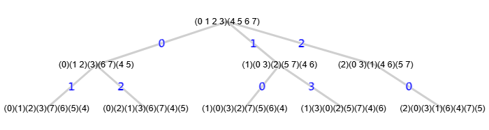
En la Figura vemos su árbol de particiones con 9 nodos y a continuación el test de isomorfismos con todas las 8! = 40320 permutaciones del grafo resultando isomórficas.
Time: 3565 ms

Test isomorfismos (McKay): {"useRefine":true,"orderRefine":"neighbors-asc-lengths-desc","typeCanon":"edges","targetCell":"first","useMcr":true,"useMcrPlus":false,"useMcrBreak":false,"typeIndicator":"none",
"isomorphic":40320,"nonIsomorphic":0,
"firstTime":3,"minTime":0,"averageTime":0,"maxTime":3,
"iter1":14,"iter2":14,
"indexTree1":8,"indexTree2":7,
"minIndexTree":7,"maxIndexTree":8,
"refine1":9,"refine2":8,
"numAut1":3,"numAut2":2,"numAutPlus1":0,"numAutPlus2":0,
"prunningMcr1":2,"prunningMcr2":3,"prunningMcrBreak1":0,"prunningMcrBreak2":0,
"prunningIndicators1":0,"prunningIndicators2":0,
"prunningIndicators1b":0,"prunningIndicators2b":0,
"canonical":[[0,6],[0,7],[1,5],[1,7],[2,4],[2,6],[3,4],[3,5],[4,5],[4,7],[5,6],[6,7]]}
Si cambiamos la opción celda objetivo "targetCell":"first" a "targetCell":"last" obtendremos un árbol con 4 nodos cuando antes era de 9 nodos:

Este es el resultado con "targetCell":"last"
Time: 0 ms

Obtener árbol particiones (McKay): {
"useRefine":true,
    "orderRefine":"neighbors-asc-lengths-desc",
    "targetCell":"last",
    "typeCanon":"edges",
    "useMcr":true,
    "useMcrPlus":false,
    "useMcrBreak":false,
    "typeIndicator":"none",
"timeTotal":0,"timeIni":0,"timeRef":0,
"iter":5,"refine":4,"indexTree":3,
"leaves":3,
"prunningMcr":1,"prunningMcrBreak":0,
"prunningIndicators":0,"prunningIndicators2":0,
"firstCanonicalPartition":[[3],[2],[1],[0],[4],[6],[7],[5]],
"firstCanon":true,
"canonicalPartition":[[3],[2],[1],[0],[4],[6],[7],[5]],
"firstCanonicalLabel":[[0,5],[0,6],[1,6],[1,7],[2,4],[2,5],[3,4],[3,7],[4,5],[4,6],[5,7],[6,7]],
"canonicalLabel":[[0,5],[0,6],[1,6],[1,7],[2,4],[2,5],[3,4],[3,7],[4,5],[4,6],[5,7],[6,7]],
"canonicalIndicator":null,
"nodes":
[[[-1,[],[],"PA"]],
[[0,[4],[],"f*"],[0,[5],[],"=(1 2)(4 5)(6 7)"],[0,[6],[],"=(0 3)(4 6)(5 7)"]]],
"nodeBest":[1,0],
"mcr":[0,1,4],
"fixMcr":
[[[0,3],[0,1,3,4,6]],
[[1,2],[0,1,2,4,5]]],
"lastEqual":true,"rebuiltMcr":0,"nonRebuiltMcr":2,
"tree":[{"index":0,"value":"(0 1 2 3)(4 5 6 7)","parent":-1},
{"index":1,"value":"(3)(2)(1)(0)(4)(6)(7)(5)","parent":[{"index":0,"value":"4"}]},
{"index":2,"value":"(3)(1)(2)(0)(5)(7)(6)(4)","parent":[{"index":0,"value":"5"}]},
{"index":3,"value":"(0)(2)(1)(3)(6)(4)(5)(7)","parent":[{"index":0,"value":"6"}]}],
"automorphisms":
[[[0],[1,2],[3],[4,5],[6,7]],
[[0,3],[1],[2],[4,6],[5,7]]],
"automorphismsPlus":0}
Y el test isomorfismos también conforme.
Time: 2234 ms

Test isomorfismos (McKay): {"useRefine":true,"orderRefine":"neighbors-asc-lengths-desc","typeCanon":"edges","targetCell":"last","useMcr":true,"useMcrPlus":false,"useMcrBreak":false,"typeIndicator":"none",
"isomorphic":40320,"nonIsomorphic":0,
"firstTime":0,"minTime":0,"averageTime":0,"maxTime":1,
"iter1":5,"iter2":5,
"indexTree1":3,"indexTree2":3,
"minIndexTree":3,"maxIndexTree":3,
"refine1":4,"refine2":4,
"numAut1":2,"numAut2":2,"numAutPlus1":0,"numAutPlus2":0,
"prunningMcr1":1,"prunningMcr2":1,"prunningMcrBreak1":0,"prunningMcrBreak2":0,
"prunningIndicators1":0,"prunningIndicators2":0,
"prunningIndicators1b":0,"prunningIndicators2b":0,
"canonical":[[0,5],[0,6],[1,6],[1,7],[2,4],[2,5],[3,4],[3,7],[4,5],[4,6],[5,7],[6,7]]}
En la siguiente tabla resumimos las combinaciones de las opciones orden refinamiento "orderRefine" y celda objetivo "targetCell" para ese grafo:
| Order refine | Target cell | ||||||
|---|---|---|---|---|---|---|---|
| first | last | max- length- first | max- length- last | min- length- first | min- length- last | max- joins | |
| neighbors-desc- lengths-desc | 4 | 9 | 4 | 9 | 4 | 9 | 4 |
| neighbors-desc- lengths-asc | 4 | 9 | 4 | 9 | 4 | 9 | 4 |
| neighbors-desc | 4 | 9 | 4 | 9 | 4 | 9 | 4 |
| neighbors-asc- lengths-desc | 9 | 4 | 9 | 4 | 9 | 4 | 9 |
| neighbors-asc- lengths-asc | 9 | 4 | 9 | 4 | 9 | 4 | 9 |
| neighbors-asc | 9 | 4 | 9 | 4 | 9 | 4 | 9 |
Estas opciones también influyen sobre el etiquetado canónico. A continuación vemos la particiones canónicas obtenidas según las celdas objetivo para dos órdenes refinamiento.
orderRefine = neighbors-asc-lengths-desc
targetCell          canonicalPartition
-----------------------------------------------------
first               [[1],[0],[3],[2],[7],[5],[6],[4]]
last                [[3],[2],[1],[0],[4],[6],[7],[5]]
max-length-first    [[1],[0],[3],[2],[7],[5],[6],[4]]
max-length-last     [[3],[2],[1],[0],[4],[6],[7],[5]]
min-length-first    [[1],[0],[3],[2],[7],[5],[6],[4]]
min-length-last     [[3],[2],[1],[0],[4],[6],[7],[5]]
max-joins           [[1],[0],[3],[2],[7],[5],[6],[4]]

orderRefine = neighbors-desc-lengths-desc
targetCell          canonicalPartition
-----------------------------------------------------
first               [[4],[7],[6],[5],[1],[0],[3],[2]]
last                [[4],[6],[5],[7],[1],[0],[3],[2]]
max-length-first    [[4],[7],[6],[5],[1],[0],[3],[2]]
max-length-last     [[4],[6],[5],[7],[1],[0],[3],[2]]
min-length-first    [[4],[7],[6],[5],[1],[0],[3],[2]]
min-length-last     [[4],[6],[5],[7],[1],[0],[3],[2]]
max-joins           [[4],[7],[6],[5],[1],[0],[3],[2]]
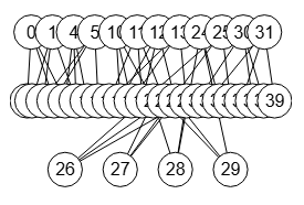
Con el grafo Miyazaki de 40 nodos de la Figura (graph-mz-2.txt) el árbol de menor tamaño se consigue con las opciones orden refinamiento neighbors-desc-lengths-desc" y celda objetivo max-joins, como vemos en la siguiente tabla:
| Order refine | Target cell | ||||||
|---|---|---|---|---|---|---|---|
| first | last | max- length- first | max- length- last | min- length- first | min- length- last | max- joins | |
| neighbors-desc- lengths-desc | 191 | 99 | 142 | 99 | 201 | 148 | 76 |
| neighbors-desc- lengths-asc | 171 | 145 | 98 | 88 | 171 | 310 | 101 |
| neighbors-desc | 179 | 124 | 86 | 76 | 179 | 275 | 89 |
| neighbors-asc- lengths-desc | 135 | 153 | 86 | 117 | 299 | 152 | 94 |
| neighbors-asc- lengths-asc | 170 | 224 | 98 | 151 | 172 | 343 | 101 |
| neighbors-asc | 129 | 149 | 86 | 117 | 289 | 149 | 94 |
Ejecutamos con esas opciones y pasamos el test isomorfismos para 16343 permutaciones, el máximo que puede ejecutar en 60 segundos.
Time: 13 ms

Obtener árbol particiones (McKay): {
"useRefine":true,"orderRefine":"neighbors-desc-lengths-desc","targetCell":"max-joins","typeCanon":"edges","useMcr":true,"useMcrPlus":false,"useMcrBreak":false,"typeIndicator":"none",
"timeTotal":13,"timeIni":1,"timeRef":9,
"iter":282,"refine":76,"indexTree":75,
"leaves":24,
"prunningMcr":155,"prunningMcrBreak":0,
"prunningIndicators":0,"prunningIndicators2":0,
"firstCanonicalPartition":[[0],[38],[39],[37],[36],[30],[31],[33],[32],[35],[34],[24],[25],[29],[27],[26],[28],[14],[23],[21],[22],[20],[18],[19],[10],[11],[13],[12],[17],[16],[1],[6],[15],[4],[3],[5],[9],[2],[7],[8]],
"firstCanon":false,
"canonicalPartition":[[16],[8],[9],[4],[27],[25],[35],[37],[36],[30],[31],[33],[32],[38],[39],[34],[0],[1],[3],[2],[20],[22],[24],[10],[12],[26],[14],[7],[6],[28],[29],[19],[18],[17],[21],[23],[5],[13],[11],[15]],
"firstCanonicalLabel":[[0,37],[0,38],[0,39],[1,5],[1,7],[1,10],[2,6],[2,8],[2,10],[3,5],[3,8],[3,9],[4,6],[4,7],[4,9],[5,8],[6,7],[9,12],[10,11],[11,13],[11,16],[12,14],[12,15],[13,19],[13,20],[14,20],[14,21],[15,18],[15,19],[16,18],[16,21],[17,22],[17,23],[17,33],[18,26],[19,25],[20,27],[21,24],[22,24],[22,26],[23,25],[23,27],[24,28],[25,29],[26,29],[27,28],[28,32],[29,32],[30,31],[30,34],[30,36],[31,34],[31,35],[32,35],[33,36],[33,39],[34,39],[35,38],[36,37],[37,38]],
"canonicalLabel":[[0,37],[0,38],[0,39],[1,3],[1,16],[1,18],[2,3],[2,17],[2,19],[3,26],[4,5],[4,20],[4,21],[5,6],[5,25],[6,7],[6,8],[7,9],[7,12],[8,10],[8,11],[9,12],[9,13],[10,11],[10,14],[11,13],[12,14],[13,15],[14,15],[15,22],[16,19],[16,27],[17,18],[17,28],[18,28],[19,27],[20,23],[20,29],[21,24],[21,30],[22,29],[22,30],[23,32],[23,33],[24,31],[24,33],[25,34],[25,35],[26,31],[26,32],[27,36],[28,36],[29,35],[30,34],[31,38],[32,37],[33,39],[34,38],[35,37],[36,39]],
"canonicalIndicator":null,
"nodes":
[[[-1,[],[]]],
[[0,[0],[]],[0,[1],[]],[0,[2],[]],[0,[4],[]],[0,[5],[]],[0,[6],[]],[0,[8],[]],[0,[10],[]],[0,[14],[]],[0,[15],[]],[0,[16],[]],[0,[18],[]],[0,[20],[]],[0,[24],[]],[0,[25],[]],[0,[26],[]]],
[[0,[0,10],[]],[0,[0,11],[]],[0,[0,12],[]],[1,[1,10],[]],[2,[2,10],[]],[3,[4,10],[]],[4,[5,10],[]],[5,[6,10],[]],[6,[8,10],[]],[7,[10,22],[]],[7,[10,23],[]],[8,[14,10],[]],[9,[15,10],[]],[10,[16,30],[]],[11,[18,30],[]],[12,[20,12],[]],[12,[20,13],[]],[13,[24,20],[]],[14,[25,20],[]],[15,[26,0],[]]],
[[0,[0,10,30],[]],[0,[0,10,31],[]],[0,[0,10,32],[]],[1,[0,11,30],[]],[2,[0,12,30],[]],[3,[1,10,30],[]],[4,[2,10,30],[]],[5,[4,10,30],[]],[6,[5,10,30],[]],[7,[6,10,30],[]],[8,[8,10,30],[]],[9,[10,22,30],[]],[10,[10,23,30],[]],[11,[14,10,30],[]],[12,[15,10,30],[]],[13,[16,30,0],[]],[14,[18,30,0],[]],[15,[20,12,0],[]],[16,[20,13,0],[]],[17,[24,20,0],[]],[18,[25,20,0],[]],[19,[26,0,30],[]]],
[[7,[4,10,30,0],[]],[8,[5,10,30,0],[]],[9,[6,10,30,8],[]],[10,[8,10,30,1],[]],[10,[8,10,30,2],[]],[11,[10,22,30,0],[]],[12,[10,23,30,0],[]],[13,[14,10,30,0],[]],[14,[15,10,30,0],[]],[15,[16,30,0,20],[]],[16,[18,30,0,21],[]],[16,[18,30,0,22],[]],[17,[20,12,0,30],[]],[18,[20,13,0,30],[]],[19,[24,20,0,30],[]],[20,[25,20,0,30],[]],[21,[26,0,30,10],[]]]],
"nodeBest":[4,9],
"mcr":[0,4,5,6,8,10,14,15,16,18],
"fixMcr":
[[[0,1,2,3,4,5,6,7,8,9,10,11,12,13,14,15,16,17,18,19,20,21,22,23,24,25,26,27,28,29,34,35],[0,1,2,3,4,5,6,7,8,9,10,11,12,13,14,15,16,17,18,19,20,21,22,23,24,25,26,27,28,29,30,32,34,35,36,38]],
[[0,1,2,3,4,5,6,7,8,9,10,11,12,13,14,15,16,17,18,19,20,21,22,23,24,25,26,27,28,29,34,35,36,37],[0,1,2,3,4,5,6,7,8,9,10,11,12,13,14,15,16,17,18,19,20,21,22,23,24,25,26,27,28,29,30,31,34,35,36,37,38]],
[[0,1,2,3,4,5,6,7,8,9,14,15,24,25,30,31,32,33,34,35,36,37,38,39],[0,1,2,3,4,5,6,7,8,9,10,12,14,15,16,18,20,22,24,25,26,28,30,31,32,33,34,35,36,37,38,39]],
[[0,1,2,3,4,5,6,7,8,9,14,15,16,17,24,25,26,27,30,31,32,33,34,35,36,37,38,39],[0,1,2,3,4,5,6,7,8,9,10,11,14,15,16,17,18,20,21,24,25,26,27,28,30,31,32,33,34,35,36,37,38,39]],
[[4,5,10,11,12,13,14,15,16,17,18,19,20,21,22,23,24,25,26,27,28,29,30,31,32,33,34,35,36,37,38,39],[0,2,4,5,6,8,10,11,12,13,14,15,16,17,18,19,20,21,22,23,24,25,26,27,28,29,30,31,32,33,34,35,36,37,38,39]],
[[4,5,6,7,10,11,12,13,14,15,16,17,18,19,20,21,22,23,24,25,26,27,28,29,30,31,32,33,34,35,36,37,38,39],[0,1,4,5,6,7,8,10,11,12,13,14,15,16,17,18,19,20,21,22,23,24,25,26,27,28,29,30,31,32,33,34,35,36,37,38,39]],
[[],[0,1,2,3,4,5,6,7,8,9,10,11,12,13,14,15,16,17,18,19]]],
"lastEqual":true,"rebuiltMcr":130,"nonRebuiltMcr":47,
"tree":null,
"automorphisms":7,
"automorphismsPlus":0}
Time: 62152 ms

Test isomorfismos (McKay): {"useRefine":true,"orderRefine":"neighbors-desc-lengths-desc","typeCanon":"edges","targetCell":"max-joins","useMcr":true,"useMcrPlus":false,"useMcrBreak":false,"typeIndicator":"none",
"isomorphic":16343,"nonIsomorphic":0,
"firstTime":17,"minTime":3,"averageTime":4,"maxTime":17,
"iter1":282,"iter2":282,
"indexTree1":75,"indexTree2":76,
"minIndexTree":74,"maxIndexTree":89,
"refine1":76,"refine2":77,
"numAut1":7,"numAut2":7,"numAutPlus1":0,"numAutPlus2":0,
"prunningMcr1":155,"prunningMcr2":154,"prunningMcrBreak1":0,"prunningMcrBreak2":0,
"prunningIndicators1":0,"prunningIndicators2":0,
"prunningIndicators1b":0,"prunningIndicators2b":0,
"canonical":[[0,37],[0,38],[0,39],[1,3],[1,16],[1,18],[2,3],[2,17],[2,19],[3,26],[4,5],[4,20],[4,21],[5,6],[5,25],[6,7],[6,8],[7,9],[7,12],[8,10],[8,11],[9,12],[9,13],[10,11],[10,14],[11,13],[12,14],[13,15],[14,15],[15,22],[16,19],[16,27],[17,18],[17,28],[18,28],[19,27],[20,23],[20,29],[21,24],[21,30],[22,29],[22,30],[23,32],[23,33],[24,31],[24,33],[25,34],[25,35],[26,31],[26,32],[27,36],[28,36],[29,35],[30,34],[31,38],[32,37],[33,39],[34,38],[35,37],[36,39]],
"warnings":["The graph has more than 9 nodes and only the first 9!=362880 permutations will be tested or less if the maximum time of 60 seconds is exceeded"]}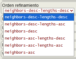
Ya explicamos las opciones orden refinamiento y celda objetivo en un tema anterior. Veamos un pequeño resumen que define cada opción.
Una partición se divide en celdas con uno o más vértices. Cada vértice del grafo tiene un determinado número de vecinos, que también denominamos como grado del vértice, vecinos que se pueden obtener con el algoritmo getNeighbors() y grados con getVertexDegrees(). Entonces cada celda tendrá una longitud que es el número de vértices que contiene y un número de vecinos que es la suma de los grados de sus vértices. Con estos dos parámetros se ordenan las particiones tras cada refinamiento:
- Orden refinamiento (
"orderRefine"):neighbors-desc-lengths-descpor número vecinos descendente primero y si hay dos iguales se ordena por longitudes también descendente.neighbors-desc-lengths-ascpor número vecinos descendente primero y si hay dos iguales se ordena por longitudes ascendente.neighbors-descpor número vecinos descendente ignorando las longitudes.neighbors-asc-lengths-descpor número vecinos ascendente primero y si hay dos iguales se ordena por longitudes descendente.neighbors-asc-lengths-ascpor número vecinos ascendente primero y si hay dos iguales se ordena por longitudes ascendente.neighbors-ascpor número vecinos ascendente ignorando las longitudes.
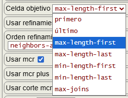
En el algoritmo que obtiene el árbol de particiones hemos de seleccionar una celda objetivo ("targetCell") de una partición no discreta con objeto de empezar a fijar vértices y refinar particiones, selección que puede obedecer a diferentes criterios. La celda que se selecciona siempre es una que contenga más de un vértice. Vea que en este momento ya tenemos una partición no discreta que previamente fue refinada y, por tanto, procede con el orden refinamiento impuesto.
- Celda objetivo (
"targetCell"):firstselecciona la primera.lastselecciona la última.max-length-firstselecciona la primera de mayor tamaño.max-length-lastselecciona la última de mayor tamaño.min-length-firstselecciona la primera de menor tamaño.min-length-lastselecciona la última de menor tamaño.max-joinsselecciona la que tenga el máximo de uniones.
La última max-joins se basa en dar a cada celda un valor en función del número de vecinos comunes con el primer vértice del resto de celdas. Es una opción costosa de obtener y que estoy probando, pues no he podido verificar una mejora en los ejemplos a excepción de algunos como el de la Figura que vimos antes.
Uso de MCR plus y corte MCR
En el tema anterior vimos el mismo grafo de la Figura que puede importar en la aplicación con graph-sample-4-plus-break.txt
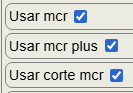
En ese tema marcábamos sólo la opción usar mcr ("useMcr") y ahora además utilizaremos usar mcr plus ("useMcrPlus") y usar corte mcr ("useMcrBreak"). Vamos a ver como estas dos opciones reducen el tamaño del árbol y el número de iteraciones respectivamente.
Vemos primero el resultado obtenido:
Time: 1 ms
Obtener árbol particiones (McKay): {
"useRefine":true,"orderRefine":"neighbors-desc-lengths-desc","targetCell":"max-length-first","typeCanon":"edges","useMcr":true,"useMcrPlus":true,"useMcrBreak":true,"typeIndicator":"none",
"timeTotal":1,"timeIni":0,"timeRef":0,
"iter":10,"refine":8,"indexTree":7,
"leaves":6,
"prunningMcr":1,"prunningMcrBreak":1,
"prunningIndicators":0,"prunningIndicators2":0,
"firstCanonicalPartition":[[0],[7],[3],[6],[2],[9],[5],[1],[8],[4]],
"firstCanon":false,
"canonicalPartition":[[1],[5],[6],[7],[4],[9],[8],[3],[2],[0]],
"firstCanonicalLabel":[[0,7],[0,8],[0,9],[1,6],[1,8],[1,9],[2,4],[2,7],[2,8],[3,5],[3,6],[3,9],[4,5],[4,7],[5,6]],
"canonicalLabel":[[0,7],[0,8],[0,9],[1,2],[1,3],[1,5],[2,4],[2,5],[3,4],[3,6],[4,9],[5,8],[6,7],[6,9],[7,8]],
"canonicalIndicator":null,
"nodes":
[[[-1,[],[],"R5","PA","PA4"]],
[[0,[0],[],"f"],[0,[1],[],">*"],[0,[2],[]],[0,[3],[],"=(0 8)(1 3)(4 7)(5 6)"],[0,[4],[],"<"]],
[[2,[2,5],[],"<"],[2,[2,6],[],"<"]]],
"nodeBest":[1,1],
"mcr":[0,1,2],
"fixMcr":
[[[2,9],[0,1,2,4,5,9]],
[[],[0,1,2,3,7]]],
"lastEqual":false,"rebuiltMcr":1,"nonRebuiltMcr":1,
"tree":[{"index":0,"value":"(0 1 2 3 4 5 6 7 8 9)","parent":-1},
{"index":1,"value":"(0)(7)(3)(6)(2)(9)(5)(1)(8)(4)","parent":[{"index":0,"value":"0"}]},
{"index":2,"value":"(1)(5)(6)(7)(4)(9)(8)(3)(2)(0)","parent":[{"index":0,"value":"1"}]},
{"index":3,"value":"(2)(5 6)(0 8)(4 7)(1 3)(9)","parent":[{"index":0,"value":"2"}]},
{"index":4,"value":"(2)(5)(6)(0)(8)(7)(4)(3)(1)(9)","parent":[{"index":3,"value":"5"}]},
{"index":5,"value":"(2)(6)(5)(8)(0)(4)(7)(1)(3)(9)","parent":[{"index":3,"value":"6"}]},
{"index":6,"value":"(3)(6)(5)(4)(7)(9)(0)(1)(2)(8)","parent":[{"index":0,"value":"3"}]},
{"index":7,"value":"(4)(8)(5)(1)(9)(2)(3)(6)(7)(0)","parent":[{"index":0,"value":"4"}]}],
"automorphisms":
[[[0,8],[1,3],[2],[4,7],[5,6],[9]]],
"automorphismsPlus":
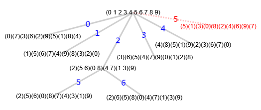
[[[0,4],[1,6],[2,9],[3,5],[7,8]]]}Y el árbol obtenido, donde agregamos la rama "5" en rojo que aparecía antes en el árbol del tema anterior y que ahora se poda por la acción de "useMcrPlus":
Antes utilizando solo "useMcr" obteníamos el árbol con 9 nodos (indexTree+1), 7 hojas (leaves), 14 iteraciones (iter) y 2 automorfismos:
...
"iter":14,"refine":9,"indexTree":8,
"leaves":7,
"prunningMcr":4,"prunningMcrBreak":0,
...
"automorphisms":
[[[0,8],[1,3],[2],[4,7],[5,6],[9]],
[[0,7],[1,5],[2,9],[3,6],[4,8]]],
"automorphismsPlus":0}
Ahora además con "useMcrPlus" y "useMcrBreak" tenemos un árbol con 8 nodos, 6 hojas, 10 iteraciones, un automorfismo (pues el otro era el de la última hoja de la rama "5" que se poda) y otro nuevo que se incluye en automorphismsPlus:
...
"iter":10,"refine":8,"indexTree":7,
"leaves":6,
"prunningMcr":1,"prunningMcrBreak":1,
...
"automorphisms":
[[[0,8],[1,3],[2],[4,7],[5,6],[9]]],
"automorphismsPlus":
[[[0,4],[1,6],[2,9],[3,5],[7,8]]]}
Para entender el efecto de "useMcrPlus" vemos a continuación el campo "nodes" puesto en forma vertical, agregando las particiones hojas:
Nº Nivel  Nodos                                       Hojas
---------------------------------------------------------------------------------
0  0      [-1,[],[],"R5","PA","PA4"]  (antes "R5","PA","PA","PA","PA"])
1  1          [[0,[0],[],"f"]                         (0)(7)(3)(6)(2)(9)(5)(1)(8)(4)
2  1          [0,[1],[],">*"]                         (1)(5)(6)(7)(4)(9)(8)(3)(2)(0)
3  1          [0,[2],[]]
4  2              [2,[2,5],[],"<"]                    (2)(5)(6)(0)(8)(7)(4)(3)(1)(9)
5  2              [2,[2,6],[],"<"]                    (2)(6)(5)(8)(0)(4)(7)(1)(3)(9)
6  1          [0,[3],[],"=(0 8)(1 3)(4 7)(5 6)"]      (3)(6)(5)(4)(7)(9)(0)(1)(2)(8)
                          (0 4)(1 6)(2 9)(3 5)(7 8)
7  1          [0,[4],[],"<"]                          (4)(8)(5)(1)(9)(2)(3)(6)(7)(0)
8  1          [0,[5],[],"=(0 7)(1 5)(2 9)(3 6)(4 8)"] (5)(1)(3)(0)(8)(2)(4)(6)(9)(7)
El algoritmo siempre usa la primera hoja como canónica (0)(7)(3)(6)(2)(9)(5)(1)(8)(4), anotada con "f", pero luego encontró que la segunda hoja (1)(5)(6)(7)(4)(9)(8)(3)(2)(0) era mayor, con lo que la marca como canónica (anotada con "<*") y que se guarda en canonicalPartition, pero sigue almacenando la primera en firstCanonicalPartition. Cuando se produzca un "=" la compara con la canónica, pero si también usamos "useMcrPlus" también la comparará con la primera canónica. Así en este ejemplo encuentra el automorfismo (0 8)(1 3)(4 7)(5 6) con la canónica y (0 4)(1 6)(2 9)(3 5)(7 8) con la primera canónica. Observamos que "5" está en el MCR (minimum cell representative) del primer automorfismo pero no del segundo. Por eso se recorta la última rama que fijaba el vértice "5" gracias a usar "usarMcrPlus".
Por otro lado con usar corte mcr ("useMcrBreak") no se reduce el tamaño del árbol, pero si el número de iteraciones. En el esquema anterior sin usar esta opción teníamos que el nodo raíz era (0 1 2 3 4 5 6 7 8 9) con cuatro podas "PA","PA","PA","PA" de los vértices 6, 7, 8, y 9, recordando que la anotación "PA" indicaba una poda por automorfismo en ese nodo. Ahora tenemos "PA","PA4", donde el primer "PA" es la poda del vértice "5" que dijimos antes por efecto de "useMcrPlus" y "PA4" son las 4 podas de los vértices 6, 7, 8, y 9 usando "useMcrBreak", que ahora se hacen todas juntas cuando entra en el primero "6", así que reduce en 4 iteraciones, de 14 antes a 10 ahora.
Comprobamos que esas opciones "useMcrPlus" y "useMcrBreak" no afectan al test de isomorfismos, al menos hasta el máximo de 362880 tests:
Time: 54069 ms

Test isomorfismos (McKay): {"useRefine":true,"orderRefine":"neighbors-desc-lengths-desc","typeCanon":"edges","targetCell":"max-length-first","useMcr":true,"useMcrPlus":true,"useMcrBreak":true,"typeIndicator":"none",
"isomorphic":362880,"nonIsomorphic":0,
"firstTime":4,"minTime":0,"averageTime":0,"maxTime":10,
"iter1":10,"iter2":10,
"indexTree1":7,"indexTree2":7,
"minIndexTree":6,"maxIndexTree":10,
"refine1":8,"refine2":8,
"numAut1":1,"numAut2":2,"numAutPlus1":1,"numAutPlus2":0,
"prunningMcr1":1,"prunningMcr2":1,"prunningMcrBreak1":1,"prunningMcrBreak2":1,
"prunningIndicators1":0,"prunningIndicators2":0,
"prunningIndicators1b":0,"prunningIndicators2b":0,
"canonical":[[0,7],[0,8],[0,9],[1,2],[1,3],[1,5],[2,4],[2,5],[3,4],[3,6],[4,9],[5,8],[6,7],[6,9],[7,8]],
"warnings":["The graph has more than 9 nodes and only the first 9!=362880 permutations will be tested or less if the maximum time of 60 seconds is exceeded"]}
La opción "useMcrPlus" sólo se producirán en árboles con secuencias de ">*" seguida posteriormente de "=", por lo que no es muy frecuente encontrar grafos de ejemplos y, en todo caso, la mejora no es muy significativa al menos en los casos que he podido analizar.
Permutaciones a cíclica permutationsToCyclic()
Cuando comparamos los etiquetados canónicos y resultan iguales "=" entonces habremos encontrado un automorfismo. Para obtenerlo tomamos las dos particiones discretas, es decir, la canónica que habíamos almacenado previamente y la actual con la que hemos comprobado que resultan iguales, y las convertimos en una permutación cíclica, concepto que ya habíamos explicado en el tema de la serie de combinatoria, en permutaciones cíclicas, siendo entonces el automorfismo encontrado.
[[1],[3],[2]]
(1)(3)(2)
[1,3,2]
1,3,2
1 3 2
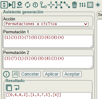
El algoritmo permutationsToCyclic() que observamos en la Figura se ejecuta en el panel del asistente de generación, al que se accede con el botón con el icono . Este algoritmo es independiente de cualquier grafo, pues solo intervienen las dos permutaciones que se van a convertir en una cíclica. Las permutaciones pueden pasarse en diversos formatos, como el ejemplo adjunto a este párrafo.
En la Figura vemos como obtenemos el automorfismo [[0,6,8,2],[1,3,7,5],[4]] a partir de las dos permutaciones (1)(3)(5)(7)(0)(2)(6)(8)(4) y (3)(7)(1)(5)(6)(0)(8)(2)(4), que son la primera partición discreta con el etiquetado canónico y la cuarta que puede verse en una tabla de un tema anterior con las 8 particiones discretas que reproducimos a continuación con todos los automorfismos que encontraba el grafo:
(1)(3)(5)(7)(0)(2)(6)(8)(4)    ()     Canónica
(1)(5)(3)(7)(2)(0)(8)(6)(4)    (0 2)(3 5)(6 8)
(3)(1)(7)(5)(0)(6)(2)(8)(4)    (1 3)(2 6)(5 7)
(3)(7)(1)(5)(6)(0)(8)(2)(4)    (0 6 8 2)(1 3 7 5)
(5)(1)(7)(3)(2)(8)(0)(6)(4)    (0 2 8 6)(1 5 7 3)
(5)(7)(1)(3)(8)(2)(6)(0)(4)    (0 8)(1 5)(3 7)
(7)(3)(5)(1)(6)(8)(0)(2)(4)    (0 6)(1 7)(2 8)
(7)(5)(3)(1)(8)(6)(2)(0)(4)    (0 8)(1 7)(2 6)(3 5)
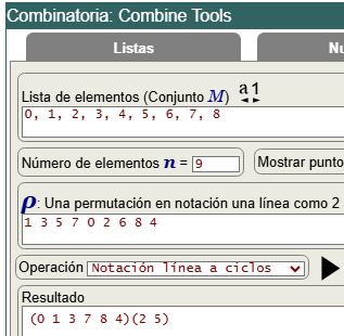
Para convertir dos permutaciones en una permutación cíclica hemos de obtener las notaciones cíclicas de cada una y obtener la división de las dos permutaciones cíclicas. Podemos usar la calculadora de permutaciones cíclicas en la aplicación Combine Tools como vemos en la Figura.
La partición discreta (1)(3)(5)(7)(0)(2)(6)(8)(4) se corresponde con la notación 1 línea en 1 3 5 7 0 2 6 8 4. Con la operación notación línea a ciclos convertimos esa permutación en 1 línea en notación cíclica (0 1 3 7 8 4)(2 5), como vemos en la Figura. Así convirtiendo a notación cíclica todas las particiones discretas y diviéndolas en esa aplicación por esa primera canónica obtenemos los mismos automorfismos que se descubren con el árbol de particiones, como vemos a continuación:
(1)(3)(5)(7)(0)(2)(6)(8)(4) ≡ 1 3 5 7 0 2 6 8 4 ≡ (0 1 3 7 8 4)(2 5) Canónica
(0 1 3 7 8 4)(2 5) ÷ (0 1 3 7 8 4)(2 5) = ()

(1)(5)(3)(7)(2)(0)(8)(6)(4) ≡ 1 5 3 7 2 0 8 6 4 ≡ (0 1 5)(2 3 7 6 8 4)
(0 1 5)(2 3 7 6 8 4) ÷ (0 1 3 7 8 4)(2 5) = (0 2)(3 5)(6 8)

(3)(1)(7)(5)(0)(6)(2)(8)(4) ≡ 3 1 7 5 0 6 2 8 4 ≡ (0 3 5 6 2 7 8 4)
(0 3 5 6 2 7 8 4) ÷ (0 1 3 7 8 4)(2 5) = (1 3)(2 6)(5 7)

(3)(7)(1)(5)(6)(0)(8)(2)(4) ≡ 3 7 1 5 6 0 8 2 4 ≡ (0 3 5)(1 7 2)(4 6 8)
(0 3 5)(1 7 2)(4 6 8) ÷ (0 1 3 7 8 4)(2 5) = (0 6 8 2)(1 3 7 5)

(5)(1)(7)(3)(2)(8)(0)(6)(4) ≡ 5 1 7 3 2 8 0 6 4 ≡ (0 5 8 4 2 7 6)
(0 5 8 4 2 7 6) ÷ (0 1 3 7 8 4)(2 5) = (0 2 8 6)(1 5 7 3)

(5)(7)(1)(3)(8)(2)(6)(0)(4) ≡ 5 7 1 3 8 2 6 0 4 ≡ (0 5 2 1 7)(4 8)
(0 5 2 1 7)(4 8) ÷ (0 1 3 7 8 4)(2 5) = (0 8)(1 5)(3 7)

(7)(3)(5)(1)(6)(8)(0)(2)(4) ≡ 7 3 5 1 6 8 0 2 4 ≡ (0 7 2 5 8 4 6)(1 3)
(0 7 2 5 8 4 6)(1 3) ÷ (0 1 3 7 8 4)(2 5) = (0 6)(1 7)(2 8)

(7)(5)(3)(1)(8)(6)(2)(0)(4) ≡ 7 5 3 1 8 6 2 0 4 ≡ (0 7)(1 5 6 2 3)(4 8)
(0 7)(1 5 6 2 3)(4 8) ÷ (0 1 3 7 8 4)(2 5) = (0 8)(1 7)(2 6)(3 5)
Observe que la primera partición que es la canónica se le asigna el automorfismo identidad, pues al dividir siempre por la primera canónica resultará la identidad (0 1 3 7 8 4)(2 5) ÷ (0 1 3 7 8 4)(2 5) = () como es obvio.
Si tenemos la partición canónica π y luego encontramos otra τ, con permutaciones cíclicas σπ y στ respectivamente, particiones cuyos etiquetados canónicos son iguales, entonces generan el automorfismo γ, de tal forma que γ = στ ÷ σπ = στ × (σπ)-1. Para el último ejemplo anterior vemos el cálculo con la inversa de la primera partición ((0 1 3 7 8 4)(2 5))-1 = (0 4 8 7 3 1)(2 5), que se obtiene manteniendo el primer índice de cada celda e invirtiendo el resto, así el cálculo con el producto resulta igual:
(0 7)(1 5 6 2 3)(4 8) ÷ (0 1 3 7 8 4)(2 5) =
(0 7)(1 5 6 2 3)(4 8) × ((0 1 3 7 8 4)(2 5))-1 =
(0 7)(1 5 6 2 3)(4 8) × (0 4 8 7 3 1)(2 5) = (0 8)(1 7)(2 6)(3 5)
En la aplicación de la calculadora de ciclos disponemos de los algoritmos para esas operaciones, una línea a ciclos para convertir la notación 1 línea en notación cíclica y división ciclos, que no es otra cosa que hacer el producto por el inverso tal como hemos dicho. Para usarlo con la obtención del árbol de particiones lo simplificamos usando el algoritmo permutationsToCyclic() que al final resulta en los mismos cálculos:
function permutationsToCyclic({permutation1=[], permutation2=[]}) {
    let dev = {error: "", cycles: []};
    try {
        let [p1, p2] = [permutation1.flat(), permutation2.flat()];
        let n = p1.length;
        if (p2.length!==n) throw new Error("Permutations lengths are wrong");
        let keys = p1.toSorted((v,w) => w-v);
        while (keys.length>0) {
            let a = keys.pop();
            let pivot = null;
            let cycle = [a];
            while (a!==pivot) {
                if (pivot===null) pivot = a;
                let i = p1.indexOf(a);
                if (i===-1) throw new Error(`i===-1`);
                let b = p2[i];
                if (b!==pivot) {
                    cycle.push(b);
                    let k = keys.indexOf(b);
                    if (k>-1) keys.splice(k, 1);
                }
                a = b;
            }
            dev.cycles.push(cycle);
        }
    } catch(e){dev.error = `#Error permutationsToCyclic(): ${e.message}`}
    return dev;
}
Vamos a seguir este algoritmo obteniendo el automorfismo (0 6 8 2)(1 3 7 5) a partir de las dos hojas discretas (1)(3)(5)(7)(0)(2)(6)(8)(4) y (3)(7)(1)(5)(6)(0)(8)(2)(4):
i =       0  1  2  3  4  5  6  7  8
p1 =     (1)(3)(5)(7)(0)(2)(6)(8)(4)
p2 =     (3)(7)(1)(5)(6)(0)(8)(2)(4)

cycles[]
keys[8,7,6,5,4,3,2,1,0]

a=0, keys=[8,7,6,5,4,3,2,1]
pivot=null, cycle=[0]
    pivot===null ⇒ pivot=a=0
    p1[4]=0 ⇒ i=4
    b=p2[4]=6
    b≠pivot ⇒ cycle=[0,6], keys=[8,7,5,4,3,2,1]
    a=b=6

    p1[6]=6 ⇒ i=6
    b=p2[6]=8
    b≠pivot ⇒ cycle=[0,6,8], keys=[7,5,4,3,2,1]
    a=b=8

    p1[7]=8 ⇒ i=7
    b=p2[7]=2
    b≠pivot ⇒ cycle=[0,6,8,2], keys=[7,5,4,3,1]
    a=b=2

    p1[5]=2 ⇒ i=5
    b=p2[5]=0
    a=b=0
    a===pivot ⇒ cycles=[[0,6,8,2]]

a=1, keys=[7,5,4,3]
pivot=null, cycle=[1]
    pivot===null ⇒ pivot=a=1
    p1[0]=1 ⇒ i=0
    b=p2[0]=3
    b≠pivot ⇒ cycle=[1,3], keys=[7,5,4]
    a=b=3

    p1[1]=3 ⇒ i=1
    b=p2[1]=7
    b≠pivot ⇒ cycle=[1,3,7], keys=[5,4]
    a=b=7

    p1[3]=7 ⇒ i=3
    bp2[3]=5
    b≠pivot ⇒ cycle=[1,3,7,5], keys=[4]
    a=b=5

    p1[2]=5 ⇒ i=2
    b=p2[2]=1
    a=b=1
    a===pivot ⇒ cycles=[[0,6,8,2],[1,3,7,5]]

a=4, keys=[]
pivot=null, cycle=[4]
    pivot===null ⇒ pivot=a=4
    p1[8]=4 ⇒ i=8
    b=p2[8]=4
    a=b=4
    a===pivot ⇒ cycles=[[0,6,8,2],[1,3,7,5],[4]]

keys=[] ⇒ cycles=[[0,6,8,2],[1,3,7,5],[4]]Código JavaScript del algoritmo básico para el etiquetado canónico con refinamiento y poda automorfismos
result = {
    canonicalPartition:null,
    canonicalLabel:null,
    nodes:[],
    mcr:null,
    fixMcr:null,
    lastEqual:false
}
A continuación vemos el pseudocódigo del algoritmo básico para obtener el etiquetado canónico con refinamiento y poda automorfismos. El resultado result contiene la partición canónica y el etiquetado canónico, con el resto de campos necesarios para la poda automorfismos. El árbol de particiones se devuelve en el campo "nodes".
Function getPartitionTreeRefineMcr(matrix, partition, result)
    If partition.length===0  // INITIAL STEPS
        partition = Initial refinement
        Add first root node to nodes
        Apply order refine
    End If
    if (partition.length===n) // DISCRETE PARTITION  (after initial refinement)
        canon = get canon with this permutation
        result.canonicalPartition = partition
        result.canonicalLabel = canon
    Else
        cell = Select target cell
        While cell.size>0
            // Fix vertex
            vertex = minimum of cell
            indexCell = position of vertex in cell
            delete vertex in cell
            filter = indexCell===0 or result.mcr===null
            If not filter
                // PRUNNING AUTORMORPHISMS
                If not lastEqual
                    result.mcr = Rebuilt MCR with result.fixMcr and node fixed path
                End If
                filter = result.mcr has vertex
            End If
            If filter
                partition = individualize vertex and refine partition
                Add new node with this fixed path to result.nodes
                If partition.length===n  // DISCRETE PARTITION
                    canon = get canon with this permutation
                    If result.canonicalLabel===null
                        result.canonicalPartition = partition
                        result.canonicalLabel = canon
                    Else
                        // Compare canon
                        If canon > result.canonicalLabel
                            result.canonicalPartition = partition
                            result.canonicalLabel = canon
                            result.lastEqual = false
                        Else if canon ===  result.canonicalLabel
                            Get automorphism with partition and result.canonicalPartition
                            and refresh result.mcr and result.fixMcr
                            result.lastEqual = true
                        Else
                            result.lastEqual = false
                        End If
                    End If
                Else
                    getPartitionTreeRefineMcr(matrix, partition, result)
                End If
            End If
        End While
    End If
    return result
End Function
El algoritmo en JavaScript básico para obtener el etiquetado canónico con refinamiento y poda automorfismos es el siguiente, versión previa a la definitiva getPartitionTree() que expondremos en otro tema. Es la misma base del que vimos en el tema anterior sólo con refinamiento, usando la misma función refinePartition() para refinar la partición.
Tenemos una función auxiliar getCanon() que ya vimos en temas anteriores para obtener el etiquetado canónico a partir de una partición discreta.
// Algorithm for get canonical label
function getCanon({matrix=[], edgesGraph=[], partition=[]}) {
    let canon = [];
    try {
        let indexes = partition.map(v => v[0]);
        let edges = edgesGraph.length>0 ? edgesGraph : matrix.edges;
        for (let edge of edges) {
            let [v, w] = edge;
            let [i, j] = [indexes.indexOf(v), indexes.indexOf(w)];
            canon.push(i<j ? [i, j] : [j, i]);
        }
        canon = canon.map(v => v[0]>v[1] ? [v[1],v[0]] : [v[0],v[1]]).toSorted((v,w) => (v[0]===w[0]) ? v[1]-w[1] : v[0]-w[0]);
    } catch(e){canon = e.message}
    return canon;
}
Y este es el algoritmo para obtener el árbol de particiones:
function getPartitionTreeRefineMcr({matrix=[], partition=[], level=-1, positionPrev=0, identity=null,
    result={canonicalPartition:null, canonicalLabel:null, nodes:[], mcr:null, fixMcr:null, lastEqual:false, automorphisms:[]}}) {
    try {
        level++;
        let n = matrix.length;
        if (partition.length===0) {
            // Initial refinement
            for (let index=0; index<n; index++) {
                let num = matrix.neighbors[index].length;
                let j = partition.findIndex(v => v.num===num);
                if (j===-1) {
                    j = partition.length;
                    let arr = [];
                    arr.num = num;
                    partition.push(arr);
                }
                partition[j].push(index);
            }
            // Add first root node to nodes
            result.nodes.push([[-1, []]]);
            // For use with fixMcr
            identity = new Set(Array.from({length:n}, (v,i)=>i));
            // orderRefine (neighbors-desc-length-desc)
            partition.sort((v,w) => v.length===w.length ?  w.num-v.num : w.length-v.length);
        }
        if (partition.length===n) { // DISCRETE PARTITION  (after initial refinement)
            // Get canon with this permutation;
            if (temp = getCanon({matrix, partition}), typeof temp==="string") throw new Error(temp);
            result.canonicalLabel = temp;
            result.canonicalPartition = partition;
        } else {
            // Select target cell (max-length-first)
            let parts = partition.map((v,i) => [i, v]).filter(v => v[1].length>1);
            let [iMax, len] = [-1, 0];
            for (let j=0; j<parts.length; j++) {
                let [i,v] = parts[j];
                let vl = v.length;
                if (vl>len) [iMax, len] = [i, vl];
            }
            let index = iMax;
            if (index>-1) {
                let cell = partition[index];
                let sCell = new Set(cell);
                while (sCell.size>0) {
                    // Fix vertex
                    let vertex = Math.min(...sCell);
                    let indexCell = cell.indexOf(vertex);
                    sCell.delete(vertex);
                    let filter =  indexCell===0 || result.mcr===null;
                    if (!filter) {
                        if (!result.lastEqual) {
                            let f = result.nodes[level][positionPrev][1];
                            let m = identity;
                            for (let j=0; j<result.fixMcr.length; j++) {
                                let [fix, mcr] = result.fixMcr[j];
                                if (f.every(v => fix.includes(v))){
                                    m = m.intersection(mcr);
                                }
                            }
                            result.mcr = m;
                        }
                        filter = result.mcr.has(vertex);
                    }
                    if (filter) {
                        let part = partition.map(v => v.slice(0));
                        part[index] = cell.toSpliced(indexCell, 1);
                        part = part.toSpliced(index, 0, [vertex]);
                        // Refine partition
                        if (part.length<n) {
                            let cells = [[vertex]];
                            part = refinePartition({matrix, partition:part, cells});
                            if (typeof part==="string") throw new Error(part);
                        }
                        // Add node to tree nodes
                        let lv = result.nodes[level].length-1;
                        if (result.nodes.length<level+2) result.nodes.push([]);
                        let prev = result.nodes[level][lv][1];
                        let fix = [...prev, vertex];
                        result.nodes[level+1].push([lv, fix]);
                        let position = result.nodes[level+1].length-1;
                        if (part.length===n) {// DISCRETE PARTITION
                            // Get canon with this permutation
                            if (temp = getCanon({matrix, partition:part}), typeof temp==="string") throw new Error(temp);
                            let canon = temp;
                            if (result.canonicalLabel===null) {
                                result.canonicalPartition = part;
                                result.canonicalLabel = canon;
                            } else {
                                // Compare canon
                                let compCanon = 0;
                                for (let i=0; i<canon.length; i++) {
                                    if (canon[i]<result.canonicalLabel[i]) {
                                        compCanon = 1;
                                        break;
                                    } else if (canon[i]>result.canonicalLabel[i]) {
                                        compCanon = -1;
                                        break;
                                    }
                                }
                                if (compCanon===1) {
                                    result.canonicalPartition = part;
                                    result.canonicalLabel = canon;
                                    result.lastEqual = false;
                                } else if (compCanon===0) {
                                    if (temp = getAutomorphism({result, part}), typeof temp==="string") throw new Error(temp);
                                    result.lastEqual = true;
                                } else {
                                    result.lastEqual = false;
                                }
                            }
                        } else {
                            let res = getPartitionTreeRefineMcr({matrix, partition:part, level, positionPrev:position, identity, result});
                            if (typeof res==="string") throw new Error(res);
                        }
                    }
                }
            }
        }
    } catch(e){result = "getPartitionTreeRefineMcr(): " + e.message}
    return result;
}
La función getAutomorphism() usa permutationsToCyclic() que vimos en un apartado anterior para obtener el automorfismo a partir de dos particiones, actualizando los campos "mcr" y "fixMcr":
function getAutomorphism({result, part}) {
    try {
        if (temp = permutationsToCyclic({permutation1:result.canonicalPartition, permutation2:part}), temp.error) throw new Error(temp.error);
        let cyclic = temp.cycles;
        result.automorphisms.push(cyclic);
        let mcr = [];
        let fix = [];
        for (let i=0; i<cyclic.length; i++) {
            let cell = cyclic[i];
            if (cell.length===1) fix.push(cell[0]);
            mcr.push(cell[0]);
        }
        if (result.fixMcr===null) {
            result.fixMcr = [[fix, new Set(mcr)]];
        } else {
            result.fixMcr.push([fix, new Set(mcr)]);
        }
        if (result.mcr===null){
            result.mcr = new Set(mcr);
        } else {
            result.mcr = result.mcr.intersection(new Set(mcr));
        }
    } catch(e){result = "getAutomorphism(): " + e.message}
    return result;
}
Para ejecutarlo puede descargar las funciones en este archivo de texto get-partition-tree-mcr.txt, copiarlo y pegarlo en la consola del navegador ejecutándose dos posibles ejemplos que ya hemos visto en un tema anterior. Vea que le pasamos la matriz de adyacencia y adjudicamos manualmente su lista de aristas y vecinos, aunque pueden obtenerser con los algoritmos getEdges() y getNeighbors()
function runGetPartitionTreeRefineMcr(sample=1) {
    let matrix;
    if (sample===1) { // Explained in https://www.wextensible.com/temas/grafos/isomorfismos-automorfismos.html#t_prunning-automorphisms
        matrix = [[0,1,0,1,0,0,0,0,0],[1,0,1,1,1,1,0,0,0],[0,1,0,0,0,1,0,0,0],[1,1,0,0,1,0,1,1,0],[0,1,0,1,0,1,0,1,0],[0,1,1,0,1,0,0,1,1],[0,0,0,1,0,0,0,1,0],[0,0,0,1,1,1,1,0,1],[0,0,0,0,0,1,0,1,0]];
        matrix.edges = [[0,1],[0,3],[1,2],[1,3],[1,4],[1,5],[2,5],[3,4],[3,6],[3,7],[4,5],[4,7],[5,7],[5,8],[6,7],[7,8]];
        matrix.neighbors = [[1,3],[0,2,3,4,5],[1,5],[0,1,4,6,7],[1,3,5,7],[1,2,4,7,8],[3,7],[3,4,5,6,8],[5,7]];
    } else if (sample===2) { // Explained in https://www.wextensible.com/temas/grafos/isomorfismos-automorfismos.html#t_rebuiltMcr
        matrix = [[0,1,0,0,1,0,0,0,1,0],[1,0,1,1,0,0,0,0,0,0],[0,1,0,1,0,0,0,0,0,1],[0,1,1,0,0,0,0,0,1,0],[1,0,0,0,0,0,1,1,0,0],[0,0,0,0,0,0,1,1,0,1],[0,0,0,0,1,1,0,0,0,1],[0,0,0,0,1,1,0,0,1,0],[1,0,0,1,0,0,0,1,0,0],[0,0,1,0,0,1,1,0,0,0]];
        matrix.edges = [[0,1],[0,4],[0,8],[1,2],[1,3],[2,3],[2,9],[3,8],[4,6],[4,7],[5,6],[5,7],[5,9],[6,9],[7,8]];
        matrix.neighbors = [[1,4,8],[0,2,3],[1,3,9],[1,2,8],[0,6,7],[6,7,9],[4,5,9],[4,5,8],[0,3,7],[2,5,6]];
    }
    let result = getPartitionTreeRefineMcr({matrix});
    // Only for view of Sets of JavaScript with JSON.stringify
    result.mcr = [...result.mcr];
    result.fixMcr = result.fixMcr.map(v => [v[0], [...v[1]]]);
    return result;
}
/* The result should be for sample 1:

{"canonicalPartition":[[1],[3],[5],[7],[0],[2],[6],[8],[4]],
"canonicalLabel":[[0,1],[0,2],[0,4],[0,5],[0,8],[1,3],[1,4],[1,6],[1,8],[2,3],[2,5],[2,7],[2,8],[3,6],[3,7],[3,8]],
"nodes":[[[-1,[]]],[[0,[1]],[0,[3]]],[[0,[1,3]],[0,[1,5]],[1,[3,1]]]],
"mcr":[0,1,4],
"fixMcr":[[[1,4,7],[0,1,3,4,6,7]],[[0,4,8],[0,1,2,4,5,8]]],
"lastEqual":true,
"automorphisms":[
    [[0,2],[1],[3,5],[4],[6,8],[7]],
    [[0],[1,3],[2,6],[4],[5,7],[8]]
]}

And for sample 2:

{"canonicalPartition":[[1],[5],[6],[7],[4],[9],[8],[3],[2],[0]],
"canonicalLabel":[[0,7],[0,8],[0,9],[1,2],[1,3],[1,5],[2,4],[2,5],[3,4],[3,6],[4,9],[5,8],[6,7],[6,9],[7,8]],
"nodes":[[[-1,[]]],[[0,[0]],[0,[1]],[0,[2]],[0,[3]],[0,[4]],[0,[5]]],[[2,[2,5]],[2,[2,6]]]],
"mcr":[0,1,2,4],
"fixMcr":[[[2,9],[0,1,2,4,5,9]],[[],[0,1,2,3,4]]],
"lastEqual":true,
"automorphisms":[
    [[0,8],[1,3],[2],[4,7],[5,6],[9]],
    [[0,7],[1,5],[2,9],[3,6],[4,8]]
]}
*/
console.log(JSON.stringify(runGetPartitionTreeRefineMcr(2)));